Wednesday, Apr 22, 2026

Aerial image stitching
Image stitching uses multiple images with overlapping sections to create a single panoramic or high-resolution image. It is used in artistic photography, medical imaging, satellite photography and is becoming very popular with the advent of modern UAVs. Here we will give a brief explanation on one of the techniques used in the image stitching process and describe the algorithms used. We are using these techniques in our products, and since this is a rather complex subject, we hope this will help you when starting your own image processing projects.
Abstract
Like many others, we don’t have a network of satellites with high-resolution cameras at our disposal, but we do have an UAV with a camera that can take pictures. In most of our business cases, UAVs or drones are widely used in agriculture. They provide real-time data about crops, but as fields can be huge, the drone should fly very high to capture the entire section, thus sacrificing small details that can make the difference.
Capturing multiple images from a lower altitude results in much finer details, but then we have to know which image is in which part of the field - similar to something Google does with satellite photos, but on a much smaller scale. We can use software to align and combine images into a single one without losing the data and knowing where we are through a process called image stitching. We will give a brief theoretical background on how one can use SIFT and Homography matrix to combine two images and show a few examples.
SIFT
SIFT - Scale-Invariant Feature Transformation - is a feature detection algorithm. It is one of the local descriptors based on gradient vector histogram. As the name suggests, SIFT is scale-invariant as opposed to, e.g., Harris detector, so it will be able to detect features regardless of the scale used. SIFT is separated into few steps which I will describe in the following text, but if you want to read more, Lowes paper is a good source.
Extrema detection
To detect features, we need frames on which we will work. Having bigger feature requires bigger frames and vice-versa. First, we have to filter by scale-space and then calculate Laplace of Gaussian operation with different σ values (where σ is a scaling parameter). Laplace of Gaussian is detecting anomalies with different σ so for example, small Gauss kernel with small σ gives greater values for smaller angle and opposite, big Gauss kernel with big σ gives greater values for a larger angle.
Laplacian of Gaussian results in a list of (x,y,σ) values which gives us potential candidates for the keypoint at location (x,y) at the scale of σ.
Laplacian of Gaussian is often impractical because it is inefficient. Therefore SIFT uses Difference of Gaussians, which is calculated as the difference of blurred images with different σ values(σ and kσ). This process occurs on all levels of the Gaussian pyramid as shown in figure 1 below.

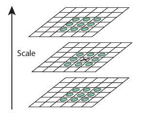
When the Difference of Gaussian is calculated, local extrema is found through scale-space. Each pixel is evaluated against its eight neighbors and nine pixels in scale value before and after, as shown in figure 2. If the pixel is a local extrema, there’s a big chance it is a keypoint or a feature.

Keypoint localization
Each keypoint from the step above is checked to get the result as accurate as possible. We use Taylor expansion of scale-space and if the intensity of the extrema is lower then the given threshold (which is 0.03 in Lowes paper), local extrema is rejected.
As a side effect, using Difference of Gaussian yields edges as keypoints as well. Edges need to be removed, so we use a concept similar to Harris edge detection called the Hessian matrix. We use 2x2 Hessian matrix to calculate curvature, and if the ratio of eigenvalues is greater then the given threshold, keypoint is rejected.
Orientation
Orientation is added to the results from the previous step. This step gives us a set of keypoints invariant to orientation. Regarding scale, a keypoint neighbor is taken, and a gradient is calculated together with a direction in the region of interest. Histogram with 36 baskets is created which covers 360 degrees. The highest and each point higher than 80% is taken for orientation calculation. The keypoint with the same location and scale is created, but with a different orientation. This contributes to the stability of finding the keypoint.
Keypoint descriptor
A descriptor is defined as a field of 16x16 pixels around a keypoint, which is then divided into 16 4x4 blocks. For each block, a histogram of 8 baskets is created, which sums to 128 baskets. The histogram is represented as a vector that forms a descriptor around a keypoint.
Once we’re done with all the steps, we can draw every keypoint over the image to see the results, which can be seen in figure 3 below.

Homography and RANSAC
The Homography matrix is used to describe the transformation between two images. To describe how one image fits the other, we need keypoint coordinates (which we got from SIFT). Homography matrix can be described by the following equation:
λ * x' = H * x
where x' is a point in the coordinate system of the transformed image, x is a point in the coordinate system of the base image, H is the homography matrix, and λ is a coefficient. If we introduce coordinates, the same equation will look like this:
λ * [x' y' 1] = H * [x y 1]
Before running the homography calculation, we need to remove the so-called outliers. As described by Marco Zuliani in his paper RANSAC For Dummies, a keypoint is considered an outlier if it doesn’t fit the “true” model instantiated by the “true” set of parameters within an error threshold that defines the maximum deviation attributable to the effects of noise.
RANSAC
RANSAC or Random Sample Consensus is an iterative method for estimating parameters of the mathematical model from the dataset. It works on dataset saturated with outliers and can work with datasets that have more than 50% of outliers. That percentage, also known as the breaking point, is the practical limitation for other algorithms (such as LMeD).
RANSAC works in two basic steps that repeat themselves; called hypothesis and test.
Hypothesis: in this step first minimal sample sets are randomly selected from the input data, and the model parameters are computed using only elements from the minimal sample set. The cardinality of minimal sample set is the smallest sufficient to determine model parameters.
Test: the second RANSAC step checks which elements of the entire dataset are consistent with the model instantiated with the parameters estimated in the first step. The set of such elements is called the consensus set.
The algorithm is finished when the probability of finding a better-ranked consensus set drops below a certain threshold. For more details on this, check Marco Zuliani’s paper.
Let’s get practical
Now that we know the theory let’s go through few examples.
For successful stitching, images require to overlap by, at least, 70%
To be sure, our images overlap by ~80%. We have captured this data using a wide-lens camera (GoPro). The problem with the GoPro camera is its lens. It produces the fish-eye effect which is terrible for the stitching, so we need to remove it. I used Adobe Lightroom (as it has predefined profiles for fish-eye removal for various GoPro cameras) to remove the fish-eye effect.


Figures 4 and 5 display a set of sample images used for stitching. These images retained their resolution even with distortion removed (that included adding artificial pixels to retain image composition and to avoid perspective distortion, all done by Adobe Lightroom).

Figure 6 displays images with completely removed distortion (that includes cropping the outer edges of the image and reducing resolution). This technique of removing outer edges yielded the best results.
Algorithm
Core requirement for the algorithm is simplicity. We take one image at the time, process it for the keypoints, do the plane transformations and add it to the final composite image. Bear in mind that the images are in 4K quality and algorithm has to scan each image. This process takes some time.
Let’s dissect the algorithm and explain what it does. We will be using OpenCV and Python. To start of, algorithm loads files from folder and is processing image by image.
We first blur black and white image using Gaussian blur with [5,5] kernel size. Afterwards we create SIFT detector and parameters for the nearest-neighbour matcher (we are using FLANN).
base_img = cv2.GaussianBlur(cv2.cvtColor(base_img_rgb,cv2.COLOR_BGR2GRAY), (5,5), 0)

#use SIFT feature detector
detector = cv2.xfeatures2d.SIFT_create()

# Parameters for nearest-neighbor matching
FLANN_INDEX_KDTREE = 1
flann_params = dict(algorithm = FLANN_INDEX_KDTREE,
    trees = 5)
matcher = cv2.FlannBasedMatcher(flann_params, {})
Right now we have prepared our base image, feature detector and matcher. What is left to do is load and prepare the next image in a row.
# Read in the next image...
next_img_rgb = cv2.imread(next_img_path)
next_img = cv2.GaussianBlur(cv2.cvtColor(next_img_rgb,cv2.COLOR_BGR2GRAY), (5,5), 0)
Images are sorted by the time of capturing thus we know that the next image will always overlap with the base by approximately 80%. Once we know that we can do the matching. (for more details see this)
# Find points in the next frame
next_features, next_descs = detector.detectAndCompute(next_img, None)

matches = matcher.knnMatch(next_descs, trainDescriptors=base_descs, k=2)
We have to filter the matches by the Lowes ratio that is lower than 0.8 (see here under Matching of local image descriptors). From there, we have to create two key point arrays from whom we will find the homography matrix. For the matching we will use RANSAC, but you can change that to LEAST_MEDIAN to see the difference.
for match in matches_subset:
    kp1.append(base_features[match.trainIdx])
    kp2.append(next_features[match.queryIdx])

p1 = np.array([k.pt for k in kp1])
p2 = np.array([k.pt for k in kp2])

H, status = cv2.findHomography(p1, p2, cv2.RANSAC, 5.0)

# how successful the transformation was
print '%d / %d  inliers/matched' % (np.sum(status), len(status))
Remember the outliers from earlier? We kind of removed them using the Lowes ratio, but RANSAC can exclude them and attempt to do the matching. The result of len(status) - np.sum(status) will give us how many outliers where there - but we don’t care about them too much.
After we calculated transformation matrix, we need to warp the images into perspective and stitch them together. We are creating a foundation image that is big enough to hold both images and then adding base image and on top the next image.
base_img_warp = cv2.warpPerspective(base_img_rgb, move_h, (img_w, img_h))
next_img_warp = cv2.warpPerspective(closestImage['rgb'], mod_inv_h, (img_w, img_h))

# Put the base image on an enlarged palette
enlarged_base_img = np.zeros((img_h, img_w, 3), np.uint8)

# Create masked composite
(ret,data_map) = cv2.threshold(cv2.cvtColor(next_img_warp, cv2.COLOR_BGR2GRAY),
    0, 255, cv2.THRESH_BINARY)

enlarged_base_img = cv2.add(enlarged_base_img, base_img_warp,
    mask=np.bitwise_not(data_map),
    dtype=cv2.CV_8U)

# Now add the warped image
final_img = cv2.add(enlarged_base_img, next_img_warp,
    dtype=cv2.CV_8U)
And we are done! Full source code can be found here.
Results!
The results are more than satisfying, taking into account how simple the algorithm is.
Figures below display the results in the same order as data samples.
Images displayed in figure 7 and 8 show a small error in the corner. This is due to lack of the keypoints in that area, so our algorithm didn’t have enough data to do the matching. Figure 9 shows the best result. That image is composed of images with no distortion, but lower in quality.
Conclusion
Implementing this kind of algorithm requires a lot of time and fine-tuning. Complex image stitching algorithms have far more features than this and are far more advanced in terms of feature detection and matching . Image stitching tools are often expensive or, if free, not available for use in enterprise environments. This blog post should give a short introduction to a simple image stitching technique that can be used to kickstart your custom projects. If you need more information, just contact us!